speeding up GPX ingest: profiling, Rcpp and furrr

a demonstration of how to profile r code on a toy problem

code performance
rstats
Author
Published

June 15, 2018

This post is a casual case study in speeding up R code. I work through several iterations of a function to read and process GPS running data from Strava stored in the GPX format. Along the way I describe how to visualize code bottlenecks with profvis and briefly touch on fast compiled code with Rcpp and parallelization with furrr.

The problem: tidying trajectories in GPX files

I record my runs on my phone using Strava. Strava stores the GPS recordings in GPX files, which are XML files that follow some additional conventions. They start with some metadata and then contain a list of GPS readings taken at one second intervals with longitude, latitude, elevation and timestap information. I wanted to approximate my speed at each timestamp in the GPS record, as well as my distance traveled since the previous GPS recordings.

Below I have an example of a GPX file that contains three GPS readings. First I create a vector that contains the names off my GPX files, and then I subset to the files that contain running data. I choose to work with the third run as a canonical example, and show a subset of the recording with three GPS readings.

library(tidyverse)
library(here)

# file contain run data
act_files <- dir(here::here("post", "2018-06-15_speeding-up-gpx-ingest-profiling-rcpp-and-furrr", "2018-04-17-activities-alex"),
  full.names = TRUE
)
run_files <- act_files[str_detect(act_files, "Run")]

# example file we'll work with
fname <- run_files[3]

# subset of example
all <- read_lines(fname)
mini_idx <- c(1:20, 5897:5899)
cat(all[mini_idx], sep = "\n")
<?xml version="1.0" encoding="UTF-8"?>
<gpx creator="StravaGPX Android" version="1.1" xmlns="http://www.topografix.com/GPX/1/1" xmlns:xsi="http://www.w3.org/2001/XMLSchema-instance" xsi:schemaLocation="http://www.topografix.com/GPX/1/1 http://www.topografix.com/GPX/1/1/gpx.xsd">
 <metadata>
  <time>2017-10-31T17:58:22Z</time>
 </metadata>
 <trk>
  <name>analytically slow</name>
  <trkseg>
   <trkpt lat="29.7169490" lon="-95.3978210">
    <ele>14.1</ele>
    <time>2017-10-31T17:58:22Z</time>
   </trkpt>
   <trkpt lat="29.7168040" lon="-95.3977180">
    <ele>14.4</ele>
    <time>2017-10-31T17:58:29Z</time>
   </trkpt>
   <trkpt lat="29.7167480" lon="-95.3976890">
    <ele>14.5</ele>
    <time>2017-10-31T17:58:30Z</time>
   </trkpt>
  </trkseg>
 </trk>
</gpx>

The part we want is in the <trkseg> tags. We’d like to turn this into a tidy dataframe where each row represents one GPS reading and the columns contain information like speed, distance, traveled, elevation gained, etc.

GPX reader version 0: using plotKML::readGPX

Note

plotKML was archived from CRAN on 2022-04-18 and the archived version isn’t easy to install. I’ve pulled the source for the readGPX() function and inserted it below to avoid depending on the plotKML package as of 2022-04-29.

Code
library(XML)

readGPX <- function(gpx.file,
                    metadata = TRUE,
                    bounds = TRUE,
                    waypoints = TRUE,
                    tracks = TRUE,
                    routes = TRUE) {
  opt <- options(warn = -1)
  if (!file.exists(gpx.file)) stop("The file '", gpx.file, "'\n  does not exist in ", getwd())

  if (metadata == TRUE) {
    metadata <- .readGPX.element(gpx.file, "name")
  }
  if (bounds == TRUE) {
    bounds <- .readGPX.element(gpx.file, "bounds")
  }
  if (waypoints == TRUE) {
    waypoints <- .readGPX.element(gpx.file, "wpt")
  }
  if (tracks == TRUE) {
    tracks <- .readGPX.element(gpx.file, "trk")
  }
  if (routes == TRUE) {
    routes <- .readGPX.element(gpx.file, "rte")
  }

  gpx <- list(metadata = metadata, bounds = bounds, waypoints = waypoints, tracks = tracks, routes = routes)
  return(gpx)
  on.exit(options(opt))
}

## Read various elements from a *.gpx file:

.readGPX.element <- function(gpx.file, element) {
  # element = "metadata", "wpt", "rte", "trk"

  ret <- xmlTreeParse(gpx.file, useInternalNodes = TRUE)
  # top structure:
  top <- xmlRoot(ret)

  # check if there is any content:
  if (any(grep(element, names(top)))) {

    # tracks:
    if (element == "trk") {
      ret <- NULL
      nu <- which(names(top) %in% element)
      for (c in seq_along(nu)) {
        lst <- which(names(top[[nu[c]]]) %in% "trkseg")
        nm <- names(top[[nu[c]]][[lst[1]]][[1]])
        ret[[c]] <- list(NULL)
        for (i in seq_along(lst)) {
          trkpt <- top[[nu[c]]][[lst[i]]]
          ret[[c]][[i]] <- data.frame(NULL)
          ## get columns (https://www.topografix.com/GPX/1/1/#type_wptType)
          lon <- as.numeric(xmlSApply(trkpt, xmlGetAttr, "lon"))
          lat <- as.numeric(xmlSApply(trkpt, xmlGetAttr, "lat"))
          ret[[c]][[i]][1:length(lon), "lon"] <- lon
          ret[[c]][[i]][1:length(lat), "lat"] <- lat
          if (!nm[[1]] == "NULL") {
            for (j in 1:length(nm)) {
              xm <- as.character(sapply(sapply(xmlChildren(trkpt), function(x) x[[nm[[j]]]]), xmlValue))
              ret[[c]][[i]][1:length(xm), nm[[j]]] <- xm
            }
          }
        }
        names(ret[[c]]) <- xmlValue(top[[nu[c]]][["name"]])
      }
    }

    if (element == "wpt") {
      ret <- data.frame(NULL)
      nu <- which(names(top) %in% element)
      nm <- names(top[[nu[1]]])
      for (i in seq_along(nu)) {
        # coordinates:
        ret[i, "lon"] <- as.numeric(xmlGetAttr(top[[nu[i]]], "lon"))
        ret[i, "lat"] <- as.numeric(xmlGetAttr(top[[nu[i]]], "lat"))
        if (!nm[[1]] == "NULL") {
          for (j in 1:length(nm)) {
            ret[i, nm[[j]]] <- xmlValue(xmlChildren(top[[nu[i]]])[[nm[[j]]]])
          }
        }
      }
    }

    if (element == "rte") {
      ret <- NULL
      nu <- which(names(top) %in% element)
      for (c in seq_along(nu)) {
        ret[[c]] <- data.frame(NULL)
        lst <- which(names(top[[nu[c]]]) %in% "rtept")
        nm <- names(top[[nu[c]]][[lst[1]]])
        for (i in seq_along(lst)) {
          rtept <- top[[nu[c]]][[lst[i]]]
          ret[[c]][i, "lon"] <- as.numeric(xmlGetAttr(rtept, "lon"))
          ret[[c]][i, "lat"] <- as.numeric(xmlGetAttr(rtept, "lat"))
          if (!nm[[1]] == "NULL") {
            for (j in c("name", "cmt", "desc", "sym", "type")) {
              try(ret[[c]][i, j] <- xmlValue(rtept[[j]]), silent = TRUE)
            }
          }
        }
        names(ret)[c] <- xmlValue(top[[nu[c]]][["name"]])
      }
    }

    # bounds
    if (element == "bounds") {
      nu <- which(names(top) %in% element)
      ret <- matrix(rep(NA, 4), nrow = 2, dimnames = list(c("lat", "lon"), c("min", "max")))
      # coordinates:
      ret[1, 1] <- as.numeric(xmlGetAttr(top[[nu[1]]], "minlon"))
      ret[1, 2] <- as.numeric(xmlGetAttr(top[[nu[1]]], "maxlon"))
      ret[2, 1] <- as.numeric(xmlGetAttr(top[[nu[1]]], "minlat"))
      ret[2, 2] <- as.numeric(xmlGetAttr(top[[nu[1]]], "maxlat"))
    }

    # metadata
    if (element == "name") {
      lst <- c("name", "desc", "author", "email", "url", "urlname", "time")
      nu <- which(names(top) %in% lst)
      if (!nu[[1]] == "NULL") {
        ret <- data.frame(NULL)
        for (i in seq_along(lst)) {
          try(ret[1, lst[i]] <- xmlValue(top[[nu[[i]]]]), silent = TRUE)
        }
      }
    }
  } else {
    ret <- NULL
  }

  return(ret)
}

Using plotKML::readGPX we can read the representative file into R.

gps_raw <- readGPX(fname)$tracks[[1]][[1]]  |> 
  as_tibble()

gps_raw
# A tibble: 1,472 × 4
     lon   lat ele   time                
   <dbl> <dbl> <chr> <chr>               
 1 -95.4  29.7 14.1  2017-10-31T17:58:22Z
 2 -95.4  29.7 14.4  2017-10-31T17:58:29Z
 3 -95.4  29.7 14.5  2017-10-31T17:58:30Z
 4 -95.4  29.7 14.6  2017-10-31T17:58:31Z
 5 -95.4  29.7 14.6  2017-10-31T17:58:32Z
 6 -95.4  29.7 14.7  2017-10-31T17:58:33Z
 7 -95.4  29.7 14.7  2017-10-31T17:58:34Z
 8 -95.4  29.7 14.7  2017-10-31T17:58:36Z
 9 -95.4  29.7 14.7  2017-10-31T17:58:37Z
10 -95.4  29.7 14.7  2017-10-31T17:58:38Z
# … with 1,462 more rows

Now we can we correct the type information:

library(lubridate)

retyped <- gps_raw |>
  mutate_at(vars(lon, lat, ele), as.numeric) |>
  mutate_at(vars(time), lubridate::ymd_hms)

retyped
# A tibble: 1,472 × 4
     lon   lat   ele time               
   <dbl> <dbl> <dbl> <dttm>             
 1 -95.4  29.7  14.1 2017-10-31 17:58:22
 2 -95.4  29.7  14.4 2017-10-31 17:58:29
 3 -95.4  29.7  14.5 2017-10-31 17:58:30
 4 -95.4  29.7  14.6 2017-10-31 17:58:31
 5 -95.4  29.7  14.6 2017-10-31 17:58:32
 6 -95.4  29.7  14.7 2017-10-31 17:58:33
 7 -95.4  29.7  14.7 2017-10-31 17:58:34
 8 -95.4  29.7  14.7 2017-10-31 17:58:36
 9 -95.4  29.7  14.7 2017-10-31 17:58:37
10 -95.4  29.7  14.7 2017-10-31 17:58:38
# … with 1,462 more rows

We want to compare location at \(t\) and \(t - 1\), so we create a lagged column of longitudes and latitudes. We put longitude and latitude together into a vector to play well with raster::pointDistance, which we’ll use to compute the great circle distance between two points.

lagged <- retyped |>
  mutate(
    x = map2(lon, lat, c), # create lagged position, this means the
    x_old = lag(x),        # first row isn't complete
    t_old = lag(time)
  ) |>
  slice(-1) # remove incomplete first row

lagged
# A tibble: 1,471 × 7
     lon   lat   ele time                x         x_old     t_old              
   <dbl> <dbl> <dbl> <dttm>              <list>    <list>    <dttm>             
 1 -95.4  29.7  14.4 2017-10-31 17:58:29 <dbl [2]> <dbl [2]> 2017-10-31 17:58:22
 2 -95.4  29.7  14.5 2017-10-31 17:58:30 <dbl [2]> <dbl [2]> 2017-10-31 17:58:29
 3 -95.4  29.7  14.6 2017-10-31 17:58:31 <dbl [2]> <dbl [2]> 2017-10-31 17:58:30
 4 -95.4  29.7  14.6 2017-10-31 17:58:32 <dbl [2]> <dbl [2]> 2017-10-31 17:58:31
 5 -95.4  29.7  14.7 2017-10-31 17:58:33 <dbl [2]> <dbl [2]> 2017-10-31 17:58:32
 6 -95.4  29.7  14.7 2017-10-31 17:58:34 <dbl [2]> <dbl [2]> 2017-10-31 17:58:33
 7 -95.4  29.7  14.7 2017-10-31 17:58:36 <dbl [2]> <dbl [2]> 2017-10-31 17:58:34
 8 -95.4  29.7  14.7 2017-10-31 17:58:37 <dbl [2]> <dbl [2]> 2017-10-31 17:58:36
 9 -95.4  29.7  14.7 2017-10-31 17:58:38 <dbl [2]> <dbl [2]> 2017-10-31 17:58:37
10 -95.4  29.7  14.7 2017-10-31 17:58:39 <dbl [2]> <dbl [2]> 2017-10-31 17:58:38
# … with 1,461 more rows

It turns out this data is not contiguous. Strava has a feature called autopause which detects pauses in runs (for example, at a stoplight), and GPS readings during paused periods are not include in the GPX files1. GPS readings typically happen once every second. I plotted the time gaps between readings and realized that time gaps greater than three seconds between two GPS recordings indicated a pause. This lets me break the run down into a series of contigous segments:

segmented <- lagged |>
  mutate(
    rest = as.numeric(time - t_old), # seconds
    new_segment = as.numeric(rest > 3),
    segment = cumsum(new_segment)
  ) |>
  # don't want t_old to be from previous segment
  group_by(segment) |>
  slice(-1)

segmented
# A tibble: 1,464 × 10
# Groups:   segment [5]
     lon   lat   ele time                x      x_old  t_old                rest
   <dbl> <dbl> <dbl> <dttm>              <list> <list> <dttm>              <dbl>
 1 -95.4  29.7  14.5 2017-10-31 17:58:30 <dbl>  <dbl>  2017-10-31 17:58:29     1
 2 -95.4  29.7  14.6 2017-10-31 17:58:31 <dbl>  <dbl>  2017-10-31 17:58:30     1
 3 -95.4  29.7  14.6 2017-10-31 17:58:32 <dbl>  <dbl>  2017-10-31 17:58:31     1
 4 -95.4  29.7  14.7 2017-10-31 17:58:33 <dbl>  <dbl>  2017-10-31 17:58:32     1
 5 -95.4  29.7  14.7 2017-10-31 17:58:34 <dbl>  <dbl>  2017-10-31 17:58:33     1
 6 -95.4  29.7  14.7 2017-10-31 17:58:36 <dbl>  <dbl>  2017-10-31 17:58:34     2
 7 -95.4  29.7  14.7 2017-10-31 17:58:37 <dbl>  <dbl>  2017-10-31 17:58:36     1
 8 -95.4  29.7  14.7 2017-10-31 17:58:38 <dbl>  <dbl>  2017-10-31 17:58:37     1
 9 -95.4  29.7  14.7 2017-10-31 17:58:39 <dbl>  <dbl>  2017-10-31 17:58:38     1
10 -95.4  29.7  14.6 2017-10-31 17:58:40 <dbl>  <dbl>  2017-10-31 17:58:39     1
# … with 1,454 more rows, and 2 more variables: new_segment <dbl>,
#   segment <dbl>

Now I calculate some information about each time point and segment that I’ll use in downstream analyses:

lonlat_dist <- partial(raster::pointDistance, lonlat = TRUE)

useful <- segmented |>
  mutate(
    seg_length = max(time) - min(t_old),  # seconds
    dx = map2_dbl(x, x_old, lonlat_dist), # meters
    dx = 0.000621371 * dx,                # miles
    dt = rest / 60^2,                     # hours
    speed = dx / dt,                      # mph
    pace = 60 * dt / dx,                  # min / mile
    elev = as.numeric(ele)                # feet
  ) |> 
  dplyr::select(-ele, -x, -x_old, -t_old, -new_segment, -rest) |>
  ungroup()

useful
# A tibble: 1,464 × 10
     lon   lat time                seg…¹ seg…²      dx      dt speed  pace  elev
   <dbl> <dbl> <dttm>              <dbl> <drt>   <dbl>   <dbl> <dbl> <dbl> <dbl>
 1 -95.4  29.7 2017-10-31 17:58:30     1 510 … 0.00423 2.78e-4 15.2   3.94  14.5
 2 -95.4  29.7 2017-10-31 17:58:31     1 510 … 0.00367 2.78e-4 13.2   4.54  14.6
 3 -95.4  29.7 2017-10-31 17:58:32     1 510 … 0.00197 2.78e-4  7.11  8.44  14.6
 4 -95.4  29.7 2017-10-31 17:58:33     1 510 … 0.00483 2.78e-4 17.4   3.45  14.7
 5 -95.4  29.7 2017-10-31 17:58:34     1 510 … 0.00230 2.78e-4  8.28  7.25  14.7
 6 -95.4  29.7 2017-10-31 17:58:36     1 510 … 0.00410 5.56e-4  7.38  8.13  14.7
 7 -95.4  29.7 2017-10-31 17:58:37     1 510 … 0.00243 2.78e-4  8.75  6.86  14.7
 8 -95.4  29.7 2017-10-31 17:58:38     1 510 … 0.00316 2.78e-4 11.4   5.27  14.7
 9 -95.4  29.7 2017-10-31 17:58:39     1 510 … 0.00415 2.78e-4 15.0   4.01  14.7
10 -95.4  29.7 2017-10-31 17:58:40     1 510 … 0.00363 2.78e-4 13.1   4.60  14.6
# … with 1,454 more rows, and abbreviated variable names ¹​segment, ²​seg_length

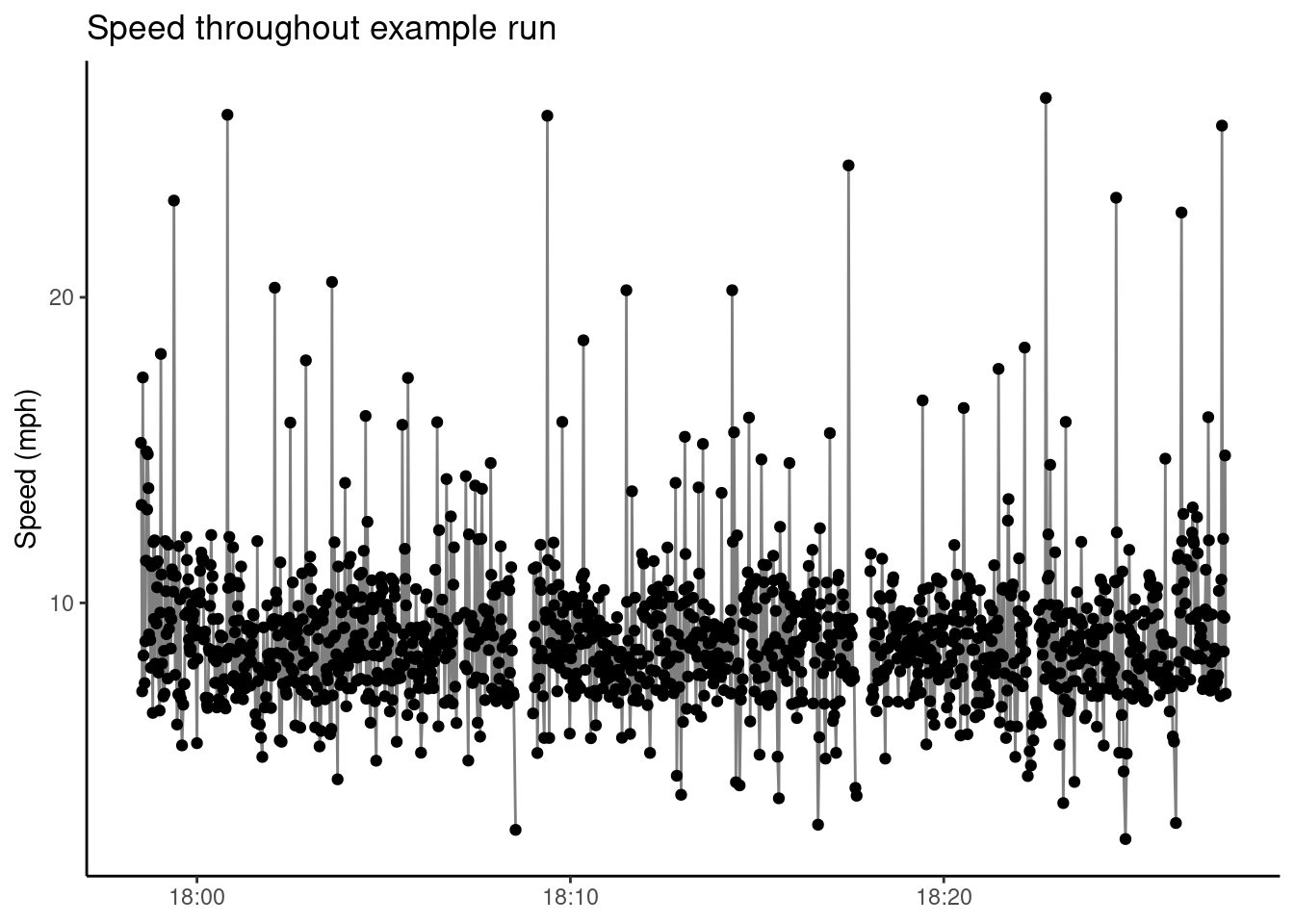
We can quickly visualize instantaneous speed throughout the run:

ggplot(useful, aes(time, speed, group = segment)) +
  geom_point() +
  geom_line(alpha = 0.5) +
  labs(
    title = "Speed throughout example run",
    y = "Speed (mph)"
  ) +
  theme_classic() +
  theme(axis.title.x = element_blank())

We can see two short pauses present in the run at around 18:08 and 18:17.

We’re going to use the code above a whole bunch, so we wrap it up into a helper function. I’m not sure that raster::pointDistance is the best option for calculating the distance between two points, so we use a dist_func argument to make it easy to switch out.

get_metrics <- function(gps_df, dist_func = lonlat_dist) {
  gps_df |>
    mutate_at(vars(lon, lat, ele), as.numeric) |>
    mutate_at(vars(time), lubridate::ymd_hms) |>
    mutate(
      x = map2(lon, lat, c),
      x_old = lag(x),
      t_old = lag(time)
    ) |>
    slice(-1) |>
    mutate(
      rest = as.numeric(time - t_old),
      new_segment = as.numeric(rest > 3),
      segment = cumsum(new_segment) + 1
    ) |>
    group_by(segment) |>
    slice(-1) |>
    mutate(
      seg_length = max(time) - min(t_old),
      dx = map2_dbl(x, x_old, dist_func),
      dx = 0.000621371 * dx,
      dt = rest / 60^2,
      speed = dx / dt,
      pace = 60 * dt / dx,
      elev = as.numeric(ele)
    ) |>
    dplyr::select(-ele, -x, -x_old, -t_old, -new_segment, -rest) |>
    ungroup()
}

This means our initial read_gpx function is just two lines:

read_gpx0 <- function(fname) {
  gps_df <- readGPX(fname)$tracks[[1]][[1]]
  get_metrics(gps_df)
}

We can use profvis::profvis to create an interactive visualization of how long it takes to read the example file.

library(profvis)

profvis(read_gpx0(fname))

In the default view, the horizontal axis represents time and the box represents the call stack. All the boxes above plotKML::readGPX are functions called by plotKML::readGPX. Here it seems like plotKML::readGPX takes about 400 milliseconds to run. So about half the time is spent reading in the file, and half calculating metrics. Most of the time calculating metrics is in raster::pointDistance, which is fairly up the call stack - you may have to click and drag the plot to see it.

GPX reader version 1: no more plotKML::GPX

Then I broke my R library and couldn’t use plotKML::readGPX for a little while. Since GPX files are XML files, I used the xml2 package as a replacement. xml2 has a function as_list that let me treat the XML as an R list. We extract the relevant portion of the list and purrr::map_dfr each GPS recording into a row of a tibble.

library(xml2)

run_xml <- read_xml(fname)
run_list <- as_list(run_xml)
gps_pts <- run_list$gpx$trk$trkseg

extract_gps_point <- function(point) {
  tibble(
    lon = attr(point, "lon"),
    lat = attr(point, "lat"),
    ele = point$ele[[1]],
    time = point$time[[1]]
  )
}

map_dfr(gps_pts, extract_gps_point)
# A tibble: 1,472 × 4
   lon         lat        ele   time                
   <chr>       <chr>      <chr> <chr>               
 1 -95.3978210 29.7169490 14.1  2017-10-31T17:58:22Z
 2 -95.3977180 29.7168040 14.4  2017-10-31T17:58:29Z
 3 -95.3976890 29.7167480 14.5  2017-10-31T17:58:30Z
 4 -95.3976530 29.7167050 14.6  2017-10-31T17:58:31Z
 5 -95.3976600 29.7166770 14.6  2017-10-31T17:58:32Z
 6 -95.3976330 29.7166110 14.7  2017-10-31T17:58:33Z
 7 -95.3976090 29.7165850 14.7  2017-10-31T17:58:34Z
 8 -95.3975830 29.7165300 14.7  2017-10-31T17:58:36Z
 9 -95.3975780 29.7164950 14.7  2017-10-31T17:58:37Z
10 -95.3975630 29.7164510 14.7  2017-10-31T17:58:38Z
# … with 1,462 more rows

Then we wrap this in a function.

read_gpx1 <- function(fname) {
  run_xml <- read_xml(fname)
  run_list <- as_list(run_xml)

  extract_gps_point <- function(point) {
    tibble(
      lon = attr(point, "lon"),
      lat = attr(point, "lat"),
      ele = point$ele[[1]],
      time = point$time[[1]]
    )
  }

  gps_df <- map_dfr(run_list$gpx$trk$trkseg, extract_gps_point)
  get_metrics(gps_df)
}

The next part is critical when trying to speed up code: test that the new code does the same thing as the old code.

library(testthat)

expected <- read_gpx0(fname)
result_1 <- read_gpx1(fname)

# silence means everything went well
expect_equal(expected, result_1)

This turned out to be too slow, so we profile and see which lines are taking the most amount of time.

profvis(read_gpx1(fname))

Here we see that we spend most of our time on the functions as_list and tibble.

GPX reader version 2: no more tibble

tibbles are somewhat heavy objects, and we can bind lists together instead of tibbles, so let’s try that next. We only change one line from read_gpx1.

read_gpx2 <- function(fname) {
  run_xml <- read_xml(fname)
  run_list <- as_list(run_xml)

  extract_gps_point <- function(point) {
    list(
      lon = attr(point, "lon"),
      lat = attr(point, "lat"),
      ele = point$ele[[1]],
      time = point$time[[1]]
    )
  }

  gps_df <- map_dfr(run_list$gpx$trk$trkseg, extract_gps_point)
  get_metrics(gps_df)
}

result_2 <- read_gpx2(fname)
expect_equal(expected, result_2)

Our results are still as expected, which is good. We profile again to see if we’ve done any better, which we have. Now we’re at about 1.5 seconds instead of 2.5 seconds.

profvis(read_gpx2(fname))

I needed to this for about fifty files though, so this was still slow enough to be somewhat frustrating. Now xml2::as_list is really killing us.

GPX reader version 3: now with more xml2

Luckily, we can use xml2 to manipulate the XML via a fast C package instead. For this next part I tried functions exported by xml2 until they worked and occasionally read the documentation.

read_gpx_xml <- function(fname) {
  # get the interested nodes
  run_xml <- read_xml(fname)
  trk <- xml_child(run_xml, 2)
  trkseg <- xml_child(trk, 2)
  trkpts <- xml_children(trkseg) # nodeset where each node is a GPS reading

  # get the longitude and latitude for each node
  latlon_list <- xml_attrs(trkpts)
  latlon <- do.call(rbind, latlon_list)

  # get the time and elevation for each node
  ele_time_vec <- xml_text(xml_children(trkpts))
  ele_time <- matrix(ele_time_vec, ncol = 2, byrow = TRUE)
  colnames(ele_time) <- c("ele", "time")

  as_tibble(cbind(latlon, ele_time))
}

read_gpx3 <- function(fname) {
  gps_df <- read_gpx_xml(fname) |> 
    select(lon, lat, everything())
  get_metrics(gps_df)
}

result_3 <- read_gpx3(fname)
expect_equal(expected, result_3) 

Again we see if there’s anywhere else we can speed things up:

profvis(read_gpx3(fname))

We’re way faster, taking less than half a second! Now the most time is spent on raster::pointDistance, which we call a ton of times. What does pointDistance do? It takes two pairs (lat1, lon1) and (lat2, lon2) the distance between them2.

GPX reader version 4: drop into Rcpp

Next I Googled how to perform this calculation myself and found this and this. The Rcpp implementation looks like:

#include <Rcpp.h>

using namespace Rcpp;

// [[Rcpp::export]]
double haversine_dist(const NumericVector p1, const NumericVector p2) {
  
  double lat1 = p1[0] * M_PI / 180;
  double lon1 = p1[1] * M_PI / 180;
  double lat2 = p2[0] * M_PI / 180;
  double lon2 = p2[1] * M_PI / 180;
  
  double d_lat = lat2 - lat1;
  double d_lon = lon2 - lon1;
  
  double a = pow(sin(d_lat / 2.0), 2) + 
    cos(lat1) * cos(lat2) * pow(sin(d_lon / 2.0), 2);
  double c = 2 * asin(std::min(1.0, sqrt(a)));
  
  return 6378137 * c; // 6378137 is the radius of the earth in meters
}

The haversine distance is fast to calculate at the cost of some small error, which we can see below:

p1 <- c(0, 0)
p2 <- c(1, 1)

dist_expected <- raster::pointDistance(p1, p2, lonlat = TRUE)
dist_result <- haversine_dist(p1, p2)

dist_result - dist_expected
[1] 525.9688

It turns out that “small error” on the geological scale is big error on the neighborhood run scale. Put all together, the C++ version looks like:

read_gpx4 <- function(fname) {
  gps_df <- read_gpx_xml(fname)
  get_metrics(gps_df, dist_func = haversine_dist)
}

We profile one more time:

profvis(read_gpx4(fname))

Now it takes only about 0.1 seconds, but the result isn’t accurate enough anymore. I wasn’t in the mood to implement a more precise great circle distance calculation, but hopefully this illustrates the general principle of dropping into Rcpp and also why it’s important to test when profiling.

Comparing the various GPX readers

Now we can compare how long each version takes using the bench package.

library(bench)

mark(
  read_gpx0(fname),
  read_gpx1(fname),
  read_gpx2(fname),
  read_gpx3(fname),
  read_gpx4(fname),
  iterations = 5, # how many times to run everything. 5 is very low.
  relative = TRUE,
  check = FALSE # since readgpx4 isn't right, will error without this
)
# A tibble: 5 × 6
  expression         min median `itr/sec` mem_alloc `gc/sec`
  <bch:expr>       <dbl>  <dbl>     <dbl>     <dbl>    <dbl>
1 read_gpx0(fname)  2.88   3.03      5.64      1.09     1.06
2 read_gpx1(fname) 17.1   18.3       1         1.27     1   
3 read_gpx2(fname)  4.97   4.97      3.65      1.03     1.14
4 read_gpx3(fname)  1.59   1.60     11.2       1.00     1.40
5 read_gpx4(fname)  1      1        16.9       1        1.05

Here timings are relative. We see that read_gpx4 is about ten times faster than read_gpx1 and two times faster than read_gpx0.

Embarrassing parallelization with furrr

In the end, I needed to do this for about fifty files. Since we can process each file independently of the other files, this operation is embarrassingly parallel. I actually wanted to use this data, so I didn’t use the C++ haversine distance function. We can write with a single map call to process all the files at once:

run_files_subset <- run_files[1:10]

map_dfr(run_files_subset, read_gpx3, .id = "run")
# A tibble: 11,780 × 11
   run     lon   lat time                seg…¹ seg…²      dx      dt speed  pace
   <chr> <dbl> <dbl> <dttm>              <dbl> <drt>   <dbl>   <dbl> <dbl> <dbl>
 1 1     -95.4  29.7 2017-10-29 18:31:00     2 907 … 0.00250 2.78e-4  9.00  6.67
 2 1     -95.4  29.7 2017-10-29 18:31:01     2 907 … 0.00245 2.78e-4  8.81  6.81
 3 1     -95.4  29.7 2017-10-29 18:31:02     2 907 … 0.00234 2.78e-4  8.41  7.13
 4 1     -95.4  29.7 2017-10-29 18:31:03     2 907 … 0.00289 2.78e-4 10.4   5.77
 5 1     -95.4  29.7 2017-10-29 18:31:04     2 907 … 0.00341 2.78e-4 12.3   4.88
 6 1     -95.4  29.7 2017-10-29 18:31:05     2 907 … 0.00315 2.78e-4 11.4   5.29
 7 1     -95.4  29.7 2017-10-29 18:31:06     2 907 … 0.00761 2.78e-4 27.4   2.19
 8 1     -95.4  29.7 2017-10-29 18:31:08     2 907 … 0.00244 5.56e-4  4.39 13.7 
 9 1     -95.4  29.7 2017-10-29 18:31:09     2 907 … 0.00322 2.78e-4 11.6   5.18
10 1     -95.4  29.7 2017-10-29 18:31:11     2 907 … 0.00349 5.56e-4  6.28  9.55
# … with 11,770 more rows, abbreviated variable names ¹​segment, ²​seg_length,
#   and 1 more variable: elev <dbl>

Which means we can also write this as a parallelized map call with furrr like so:

library(furrr)
plan(multiprocess, workers = 12)

future_map_dfr(run_files, read_gpx3, .id = "run")
# A tibble: 59,833 × 11
   run     lon   lat time                seg…¹ seg…²      dx      dt speed  pace
   <chr> <dbl> <dbl> <dttm>              <dbl> <drt>   <dbl>   <dbl> <dbl> <dbl>
 1 1     -95.4  29.7 2017-10-29 18:31:00     2 907 … 0.00250 2.78e-4  9.00  6.67
 2 1     -95.4  29.7 2017-10-29 18:31:01     2 907 … 0.00245 2.78e-4  8.81  6.81
 3 1     -95.4  29.7 2017-10-29 18:31:02     2 907 … 0.00234 2.78e-4  8.41  7.13
 4 1     -95.4  29.7 2017-10-29 18:31:03     2 907 … 0.00289 2.78e-4 10.4   5.77
 5 1     -95.4  29.7 2017-10-29 18:31:04     2 907 … 0.00341 2.78e-4 12.3   4.88
 6 1     -95.4  29.7 2017-10-29 18:31:05     2 907 … 0.00315 2.78e-4 11.4   5.29
 7 1     -95.4  29.7 2017-10-29 18:31:06     2 907 … 0.00761 2.78e-4 27.4   2.19
 8 1     -95.4  29.7 2017-10-29 18:31:08     2 907 … 0.00244 5.56e-4  4.39 13.7 
 9 1     -95.4  29.7 2017-10-29 18:31:09     2 907 … 0.00322 2.78e-4 11.6   5.18
10 1     -95.4  29.7 2017-10-29 18:31:11     2 907 … 0.00349 5.56e-4  6.28  9.55
# … with 59,823 more rows, abbreviated variable names ¹​segment, ²​seg_length,
#   and 1 more variable: elev <dbl>

Note that other than loading furrr and calling plan(multiprocess) all we’ve had to do to get parallelism is to call furrr::future_map_dfr, which has exactly the same API as purrr::map_dfr. My computer has twelve cores, meaning there’s a maximum possible speedup of twelve.

mark(
  sequential = map_dfr(run_files, read_gpx3, .id = "run"),
  parallel = future_map_dfr(run_files, read_gpx3, .id = "run"),
  iterations = 5,
  memory = FALSE,
  relative = TRUE
)
# A tibble: 2 × 6
  expression   min median `itr/sec` mem_alloc `gc/sec`
  <bch:expr> <dbl>  <dbl>     <dbl>     <dbl>    <dbl>
1 sequential  5.00   4.55      1           NA     1   
2 parallel    1      1         4.50        NA     4.10

Wrap Up

This was a low stakes exercise in speeding up R code. By the time I’d written all of these it would have been several hundred times faster to use read_gpx0 and just save the results to a .rds file. Still, it was fun to work through the profiling workflow and I look forward to enterprising strangers on the internet pointing out places where things can get faster still.

See also gpx for a more modern approach to reading .gpx files in R that did not exist at the time I originally wrote this blogpost.

Footnotes

  1. It took me a two months to realize this, mostly because I didn’t plot enough of the data. If you’re curous how Strava detects paused movement, you can read more here. It seems to involve more if-statements than fun models.↩︎

  2. We can’t calculate the distance using the L2 norm because longitude and latitude are spherical coordinates, not Euclidean coordinates.↩︎

Reuse