Summary
A while back Twitter once again lost its collective mind and decided to rehash the logistic regression versus linear probability model debate for the umpteenth time. The genesis for this new round of chaos was Gomila (2019), a pre-print by Robin Gomila, a grad student in psychology at Princeton.
So I decided to learn some more about the linear probability model (LPM), which has been on my todo list since Michael Weylandt suggested it as an example for a paper I’m working on. In this post I’ll introduce the LPM, and then spend a bunch of time discussing when OLS is a consistent estimator.
Update: I turned this blog post into somewhat flippant, meme-heavy slides.
What is the linear probability model?
Suppose we have outcomes \(Y \in \{0, 1\}\) and fixed covariate vectors \(X\). The linear probability model is a model, that is, a set of probability distributions that might have produced our observed data. In particular, the linear probability assumes that the data generating process looks like:
\[\begin{align} P(Y = 1 | X) = \begin{cases} 1 & \beta_0 + \beta_1 X_1 + ... + \beta_k X_k > 1 \\ \beta_0 + \beta_1 X_1 + ... + \beta_k X_k & \beta_0 + \beta_1 X_1 + ... + \beta_k X_k \in [0, 1] \\ 0 & \beta_0 + \beta_1 X_1 + ... + \beta_k X_k < 0 \end{cases} \end{align}\]
Essentially we clip \(P(Y = 1 | X) = X \beta\) to \([0, 1]\) to make sure we get valid probabilities. We can contrast the LPM with the binomial GLM, where the assumption is that:
\[\begin{align} P(Y = 1 | X) = \frac{1}{1 + \exp(-(\beta_0 + \beta_1 X_1 + ... + \beta_k X_k))} \end{align}\]
At points throughout this post we will also be interested in Gaussian GLMs. In slightly different notation, we can write all of these models as follows:
\[\begin{align} Y_i | X_i &\sim \mathrm{Bernoulli}(\min(1, \max(0, X_i \beta))) & \text{linear probability model} \\ Y_i | X_i &\sim \mathrm{Bernoulli}(\mathrm{logit}^{-1} (X_i \beta)) & \text{logistic regression / binomial GLM} \\ Y_i | X_i &\sim \mathrm{Normal}(X_i \beta, \sigma^2) & \text{linear regression / Gaussian GLM} \end{align}\]
The OLS estimator
When people refer to the linear probability model, they are referring to using the Ordinary Least Squares estimator as an estimator for \(\beta\), or using \(X \hat \beta_\text{OLS}\) as an estimator for \(\mathbb{E}(Y|X) = P(Y = 1|X)\). The OLS estimator is:
\[\begin{align} \hat \beta_\text{OLS} = (X'X)^{-1} X' Y. \end{align}\]
Most people have seen the OLS estimator derived as the MLE of a Gaussian linear model. Here we have binary data, which is definitely non-Gaussian, and this is aesthetically somewhat unappealing. The big question is whether or not using \(\hat \beta_\text{OLS}\) on binary data actually works.
A bare minimum for inference
When we do inference, we pretty much always want two things to happen. Given our model (the assumptions we are willing to make about the data generating process):
- our estimand should be identified, and
- our estimator should be consistent.
Identification means that each possible value of the estimand should correspond to a distinct distribution in our probability model. When we say that we want a consistent estimator, we mean that our estimator should recover the estimand exactly with infinite data. All the estimands in the LPM debate are identified (to my knowledge), so this isn’t the big deal here. But consistency matters a lot!
Gomila (2019) claims that \(\hat \beta_\text{OLS}\) is unbiased and consistent for \(\beta\), and attempts to demonstrate this two ways: (1) analytically, and (2) via simulation.
And this is the point that I got pretty confused, because the big question is: consistent under what model? Depending on who you ask, we could conceivably be assuming that the data comes from:
- a Gaussian GLM (linear regression),
- the linear probability model, or
- a binomial GLM (logistic regression).
Consistency of the OLS estimator
The easiest case is when we assume that a Gaussian GLM (linear regression model) holds. In this case, \(\hat \beta_\text{OLS}\) is unbiased and consistent. My preferred reference for this is Rencher and Schaalje (2008).
When the linear probability model holds, \(\hat \beta_\text{OLS}\) is in general biased and inconsistent (Horrace and Oaxaca (2003)). However, Gomila (2019) claims that OLS is unbiased and consistent. Over Twitter DM I clarified that this claim is with respect to the linear probability model. Gomila referred me to Wooldridge (2001) for an analytic proof, and to his simulation results for empirical confirmation.
At this point the main result of Horrace and Oaxaca (2003) becomes germane. It goes like this: the OLS estimator is consistent and unbiased under the linear probability model if \(X_i^T \beta \in [0, 1]\) for all \(i\), otherwise the OLS estimator is biased and inconsistent. In fact, Wooldridge (2001) makes the same point:
Unless the range of \(X\) is severely restricted, the linear probability model cannot be a good description of the population response probability \(P(Y = 1|X)\).
Here are some simulations demonstrating this bias and inconsistency when the \(X_i^T \beta \in [0, 1]\) condition is violated. It’s pretty clear that OLS is in general biased and inconsistent under the linear probability model. I was curious why this wasn’t showing up in Gomila’s simulations, so I took a look at his code and it turned out he wasn’t simulating from diverse enough data generating processes.
We discussed this over Twitter DM, and Gomila has since updated the code, but I believe the new simulations still do not seriously violate the \(X_i^T \beta \in [0, 1]\) condition. I briefly played around with the code but then it was 2 AM and I didn’t understand DeclareDesign particularly well so I gave up. Many kudos to Gomila for posting his code for public review.
Anyway, the gist is that OLS is consistent under the linear probability model if \(X_i^T \beta\) is between zero and one for all \(i\).
What if logistic regression is the true model?
Another reasonable question is: what happens to \(\hat \beta_\text{OLS}\) under a binomial GLM? The story here is pretty much the same: \(\hat \beta_\text{OLS}\) is not consistent for \(\beta\), but it often does a decent job of estimating \(\mathbb{E}(Y|X)\) anyway (Battey et al. 2019; Cox 1958).
The intuition behind this comes from M-estimation1, which we digress into momentarily. The idea is to observe that \(\hat \beta_\text{OLS}\) is an M-estimator. To see this, recall that OLS is based on minimizing
\[\begin{align*} \mathcal{L}(X, Y, \beta) = \frac 12 \Vert Y - X \beta \Vert_2^2 \end{align*}\]
which has a global minimizer \(\beta_0\). The gradient,
\[\begin{align*} \nabla \mathcal{L}(X, Y, \beta) = \left( Y - X \beta \right)' X, \end{align*}\]
should be zero at \(\beta_0\) under any model with linear expectation (provided that \(X_i \neq 0\) for all \(i\)). So we take \(\psi = \nabla \mathcal{L}(X, Y, \beta_0)\) as the function in our estimating equation, since \(\mathbb{E} (\psi) = 0\). This lets us leverage standard results from M-estimation theory.
In particular, M-estimation theory tells us that \(\hat \beta_\text{OLS}\) is consistent under any regular distribution \(F\) such that \(\beta_0\) is the unique solution to
\[\begin{align*} \mathbb{E}_F \left[ \left( Y_i - X_i^T \beta_0 \right)' X_i \right] = 0. \end{align*}\]
We can use this to derive a sufficient condition for consistency; namely OLS is consistent for \(\beta_0\) if
\[\begin{align*} 0 &= \mathbb{E}_F \left[ \left( Y - X_i^T \beta_0 \right)' X_i \right] \\ &= \mathbb{E}_F \left[ \mathbb{E}_F \left[ \left( Y - X_i^T \beta_0 \right)' X_i \Big \vert X_i \right] \right] \\ &= \mathbb{E}_F \left[ \mathbb{E}_F \left[ Y - X_i^T \beta_0 \Big \vert X_i \right]' X_i \right]. \end{align*}\]
So a sufficient condition for the consistency of OLS is that
\[\begin{align*} \mathbb{E}_F(Y | X_i) = X_i^T \beta_0. \end{align*}\]
That is, if the expectation is linear in some model parameter \(\beta_0\), OLS is consistent for that parameter. If you are an economist you’ve probably seen this written as
\[\begin{align*} \mathbb{E}_F(\varepsilon_i | X_i) = 0, \end{align*}\]
where we take \(\varepsilon_i = Y_i - \mathbb{E}(Y_i | X_i)\).
The sufficient condition is also a necessary condition, and if it is violated \(\hat \beta_\text{OLS}\) will generally be asymptotically biased.
Returning from our digression into M-estimation, we note the condition that \(\mathbb{E}_F(Y | X_i) = X_i^T \beta_0\) is shockingly weaker than the assumption we used to derive \(\hat \beta_\text{OLS}\), where we used the fact that \(Y\) followed a Gaussian distribution. For consistency, we only need an assumption on the first moment of the distribution of \(Y\), rather than the full parametric form of the model, which specifies every moment \(\mathbb{E}(Y^2), \mathbb{E}(Y^3), \mathbb{E}(Y^4), ...\) of \(Y\).
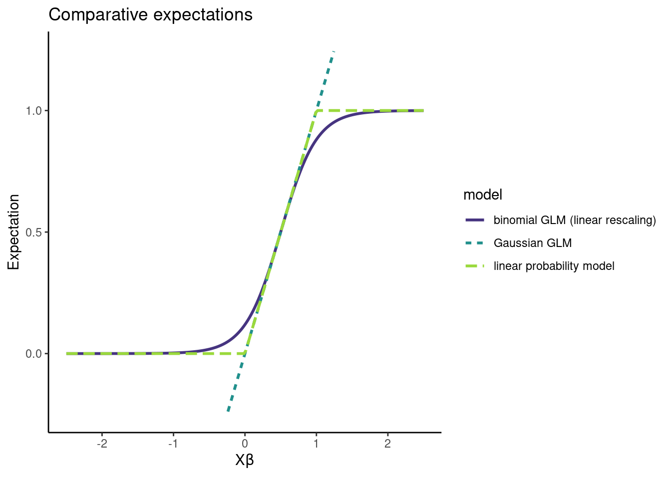
Anyway, the expectation of a binomial GLM is \(\mathrm{logit}^{-1} (X_i \beta)\), and the expectation of the LPM is \(\min(1, \max(0, X_i \beta))\). For certain \(X_i\) and \(\beta\), these expectations are very close to \(X_i \beta\). In these cases, estimates for \(\mathbb{E}(Y|X)\) based on \(\hat \beta_\text{OLS}\) will do well2.
Looking at the expectations of the models, we can see they aren’t wildly different:
Note that, under the LPM, \(\hat \beta_\text{OLS}\) can give us good estimates for \(\beta\), but under logistic regression, we only get good estimates of \(\mathbb{E}(Y|X)\)3.
So maybe don’t toss the LPM estimator out with the bath water. Sure, the thing is generally inconsistent and aesthetically offensive, but whatever, it works on occasion, and sometimes there will be other practical considerations that make this tradeoff reasonable.
Where the estimator comes from doesn’t matter
Bayes Twitter in particular had a number of fairly vocal LPM opponents, on the basis that \(\hat \beta_\text{OLS}\) was derived under a model that can’t produce the observed data.
This might seem like a dealbreaker, but it doesn’t bother me. Where the estimator comes from doesn’t actually matter. If it has nice properties given the assumptions you are willing to make, you should use it! Estimators derived under unrealistic models4 often turn out to be good!
In a bit more detail, here’s how I think of model checking:
- There’s an estimand I want to know
- I make some assumptions about my data generating process
- I pick an estimator that has nice properties given this data generating process
The issue here is that my assumptions about the data generating process can be wrong. And if my modeling assumptions are wrong, then my estimator might not have the nice properties I want it to have, and this is bad.
The concern is that using \(\hat \beta_\text{OLS}\) corresponds to making a bad modeling assumption. In particular, using a Gaussian model for binary data isn’t defensible.
That’s not really what’s going on though. Instead, we start by deriving an estimator under the linear regression model. Then, we show this estimator has nice properties under a new, different model. To do model checking, we need to test whether the new, different model holds. Whether or not the data comes from a linear regression is immaterial.
Nobody who likes using \(\hat \beta_\text{OLS}\) is arguing that it’s reasonable to assume a Gaussian generative model for binary data. LPM proponents argue that the Gaussian modeling assumption is violated, but it isn’t violated in an important way. Look, they say, the key assumptions of a Gaussian model that we used to derive consistency results can still hold, even if some other assumptions get violated. This is exactly what the M-estimation approach formalizes.
What about uncertainty in our estimator?
So far we have established that \(\hat \beta_\text{OLS}\) is at least occasionally a consistent estimator for \(P(Y=1|X)\) under the LPM and logistic regression.
In practice, we also care about the uncertainty in \(\hat \beta\). We might want a confidence interval, or, God forbid, a p-value. So we should think about consistent estimators for \(\mathbf{Cov} (\hat \beta)\). In the grand LPM debate, most people suggest using robust standard errors. For a while, it was unclear to me how these robust standard errors were derived and under what conditions they are consistent. The answer again comes from Boos and Stefanski (2013), and all we need for the consistency of robust standard errors for \(\mathbf{Cov} (\hat \beta)\) is some moment conditions (the existence of (7.5) and (7.6) in the text), which linear regression, logistic regression, and the LPM all satisfy.
It only took several weeks of misreading Boos and Stefanski (2013) and asking dumb questions on Twitter to figure this out. Thanks to Achim Zeileis, James E. Pustejovsky, Cyrus Samii for answering those questions. Note that White (1980) is another canonical paper on robust standard errors, but it doesn’t click for me like the M-estimation framework does.
Takeaways
This post exists because I wasn’t sure when \(\hat \beta_\text{OLS}\) was a consistent estimator, and the rest of the LPM debate seemed like a lot of noise until I could figure that out. I have three takeaways.
Properties of estimators are always with respect to models, and it’s hard to discuss which estimator is best if you don’t clarify modeling assumptions.
If there are multiple reasonable estimators, fit them all. If they result in substantively different conclusions: congratulations! Your data is trash and you can move on to a new project!
If you really care about getting efficient, consistent estimates under weak assumptions, you should be doing TMLE or Double ML or burning your CPU to a crisp with BART5.
Anyway, this concludes the “I taught myself about the linear probability model and hope to never mention it again” period of my life. I look forward to my mentions being a trash fire.
References
Battey, H. S., D. R. Cox, and M. V. Jackson. 2019. “On the Linear in Probability Model for Binary Data.” Royal Society Open Science 6 (5): 190067. https://doi.org/10.1098/rsos.190067.
Boos, Dennis D, and L. A Stefanski. 2013. Essential Statistical Inference. Vol. 120. Springer Texts in Statistics. Springer New York. https://doi.org/10.1007/978-1-4614-4818-1.
Cox, D. R. 1958. “The Regression Analysis of Binary Sequences.” Journal of the Royal Statistical Society. Series B (Methodological) 20 (2): 215–42. http://www.jstor.org/stable/2983890.
Gomila, Robin. 2019. Logistic or Linear? Estimating Causal Effects of Binary Outcomes Using Regression Analysis. Preprint. PsyArXiv. https://doi.org/10.31234/osf.io/4gmbv.
Horrace, William C, and Ronald L Oaxaca. 2003. New Wine in Old Bottles: A Sequential Estimation Technique for the LPM. 43. https://papers.ssrn.com/sol3/papers.cfm?abstract_id=383102.
Rencher, Alvin C., and G. Bruce Schaalje. 2008. Linear Models in Statistics. 2nd ed. Wiley-Interscience. http://www.utstat.toronto.edu/~brunner/books/LinearModelsInStatistics.pdf.
White, Halbert. 1980. “A Heteroskedasticity-Consistent Covariance Matrix Estimator and a Direct Test for Heteroskedasticity.” Econometrica 48 (4): 817. https://doi.org/10.2307/1912934.
Wooldridge, Jeffrey M. 2001. Econometric Analysis of Cross Section and Panel Data. https://mitpress.mit.edu/books/econometric-analysis-cross-section-and-panel-data-second-edition.
Footnotes
An M-estimator \(\hat \theta\) is a solution to
\[\begin{align*} \sum_{i=1}^n \psi(Y_i, \hat \theta) = 0 \end{align*}\]
for some function \(\psi\). Think of \(\psi\) as a score function or the derivative of a proper scoring rule. If the true value \(\theta_0\) is the unique solution to
\[\begin{align*} \mathbb{E} \left( \sum_{i=1}^n \psi(Y_i, \theta_0) \right) = 0 \end{align*}\]
then \(\hat \theta \to \theta_0\). So it’s relatively easy to check if an M-estimator is consistent. Additionally, under some regularity conditions, provided that
\[\begin{align*} A(\theta_0) = \mathbb{E} \left( - \psi' (Y_i, \theta_0) \right) \end{align*}\]
and
\[\begin{align*} B(\theta_0) = \mathbb{E} \left( \psi(Y_i, \theta_0) \psi(Y_i, \theta_0)^T \right) \end{align*}\]
exist for all \(i = 1, ..., n\), then \(\hat \theta\) is also asymptotically normal with variance \(A(\theta_0)^{-1} \cdot B(\theta_0) \cdot \{ A(\theta_0)^{-1} \}^T\). We also have that
\[\begin{align*} A(\hat \theta)^{-1} \cdot B(\hat \theta) \cdot \{ A(\hat \theta)^{-1} \}^T \rightarrow A(\theta_0)^{-1} \cdot B(\theta_0) \cdot \{ A(\theta_0)^{-1} \}^T \end{align*}\]
so life is pretty great and we can get asymptotic estimates of uncertainty for \(\hat \theta\).↩︎
In a lot of experimental settings that compare categorical treatments, you fit a fully saturated model that allocates a full parameter to the mean of each combination of treatments. \(\hat \beta_\text{OLS}\) is consistent in this setting under both logistic regression and the LPM.
Let’s prove this for logistic regression first. Suppose we have groups \(1, ..., k\) and the data comes from a logistic regression model. We represent the groups in the model via one hot coding, omitting an intercept for identifability. That is, we assume
\[\begin{align} P(Y = 1 | X) = \frac{1}{1 + \exp(-(\alpha_1 X_1 + ... + \alpha_k X_k))} \end{align}\]
where \(X_j = 1\) if the observation comes from group \(j\) and is zero otherwise. Note that, if \(X_j = 1\), then \(X_i = 0\) for all \(i \neq j\). To verify that the mean function is correctly specified, and thus that OLS is consistent, we need \(\mathbb{E}(Y|X) = X^T \beta\).
Put \(\beta_j = \frac{1}{1 + \exp(-\alpha_j)}\), which is the mean of the \(j^{th}\) group. Recall that \(X_j\) is fixed, so that \(P(X_j = 1) = X_j\). Then:
\[\begin{align} \mathbb{E} (Y | X) &= P(Y = 1 | X) \\ &= P(Y = 1|X_1 = 1) \cdot P(X_1 = 1) + ... + P(Y = 1|X_k = 1) \cdot P(X_k = 1) \\ &= P(Y = 1|X_1 = 1) \cdot X_1 + ... + P(Y = 1|X_k = 1) \cdot X_k \\ &= \frac{1}{1 + \exp(-\alpha_1)} \cdot X_1 + ... + \frac{1}{1 + \exp(-\alpha_k)} \cdot X_k \\ &= \beta_1 X_1 + ... + \beta_k X_k \\ &= X^T \beta \end{align}\]
Thus \(\hat \beta_\text{OLS} \to \beta\). So the OLS estimates are consistent for the group means, and \(\left(\hat \beta_\text{OLS} \right)_j \to \frac{1}{1 + \exp(-\alpha_j)}\).
Okay, now we’re halfway done but we still need to show consistency under the LPM. We assume the model is
\[\begin{align} P(Y = 1 | X) = \min(1, \max(0, \gamma_1 X_1 + ... + \gamma_k X_k)) \end{align}\]
Putting \(\beta_j = \min(1, \max(0, \gamma_j))\) we repeat the same procedure almost verbatim and see:
\[\begin{align} \mathbb{E} (Y|X) &= P(Y = 1|X) \\ &= P(Y = 1|X_1 = 1) \cdot P(X_1 = 1) + ... + P(Y = 1|X_k = 1) \cdot P(X_k = 1) \\ &= P(Y = 1|X_1 = 1) \cdot X_1 + ... + P(Y = 1|X_k = 1) \cdot X_k \\ &= \min(1, \max(0, \gamma_1)) \cdot X_1 + ... + \min(1, \max(0, \gamma_k)) \cdot X_k \\ &= \beta_1 X_1 + ... + \beta_k X_k \\ &= X^T \beta \end{align}\]
Thus \(\hat \beta_\text{OLS} \to \beta\). So the OLS estimates are again consistent for the group means \(\beta_j = \min(1, \max(0, \gamma_j))\).↩︎
Michael Weylandt suggested the following example as an illustration of this. Suppose we are going to compare just two groups, so \(X_i \in \{0, 1\}\), and the true model is \(P(Y = 1|X) = \mathrm{logit}^{-1} (1 - 2 X_i)\). Consider the infinite data limit so we don’t have to worry about estimation error.
We know that \(P(Y_i = 1 | X_i = 0) = 0.731\) and \(P(Y_i = 1 | X_i = 1) = 0.269\). \(\hat \beta_\text{logistic MLE} = \beta = (1, -2)\) by the consistency of the MLE. The OLS fit will yield \(P(Y_i = 1 | X_i) = 0.731 - 0.462 X_i\). The predictions for \(\mathbb{E}(Y|X) = P(Y=1|X)\) agree, but \(\hat \beta_\text{OLS} = (0.731, -0.4621)\) while \(\beta = (1, -2)\).
This is a concrete application of the result in the previous footnote: \(\hat \beta_\text{OLS}\) being consistent for group means only results in \(\hat \beta_\text{OLS}\) being consistent for the model parameters \(\beta\) if the model parameters are themselves the group means.↩︎
I.I.D. assumptions are often violated in real life, for example!
My advisor made an interesting point about critiquing assumptions the other day. He said that it isn’t enough to say “I don’t think that assumption holds” when evaluating a model or an estimator. Instead, to show than the assumption is unacceptable, he claims you need to demonstrate that making a particular assumption results in some form of undesirable inference.↩︎
Gomila also makes an argument against using \(\hat \beta_\text{logistic MLE}\) based on some papers that show it handles interactions poorly. This sort of misses the forest for the trees in my opinion. GLMs are generically dubious models because few empirical conditional expectations are actually linear. And maybe linear main effects won’t kill you, but modeling interactions with linear terms amounts to fitting global hyperplanes for interactions. This is undesirable because interactions are almost always local, not global. If you want to model interactions carefully, you need something flexible like a GAM or kernels or whatnot.↩︎